General Approach: Mass Spring Systems
Dynamics, in its common usage, just means change. In computer graphics it has a specialized meaning which refers to the way that objects with mass behave when subjected to forces.
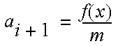
A point mass m when subjected to a force, ƒ, will experience an acceleration, a, in accordance with the following equation:

A point mass originally at rest will have an increase in velocity, v, defined by:
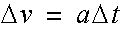
where

means increment in time and

means change in velocity.
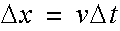
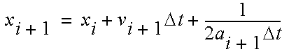
At the same time the velocity will cause a change in position:
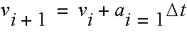
Therefore, it is possible to find the new position based on the previous position for each step. Thinking of the variables at increment i and increment i + 1:
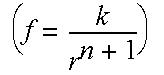
The force ƒ was shown as ƒ(x) which means that the force is a function of position, for example:
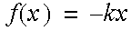
This means that a mass at positive x will experience a force pulling it towards the origin. If the mass is at negative x the mass will also be pulled towards the origin. A mass released at position x = p will oscillate around the origin. The force simulates the effect of a spring. The value of k determines how stiff the spring is. The larger the value of k, the stiffer the spring and the faster the oscillation. Experiment usinge a wireframe to create preview files. Try different values of k. The frequency will change. Try different values of mass. What effects does this have?
A mass on a perfect spring will oscillate forever. In practice, though, real world devices experience friction and atmospheric drag. This may be simulated by modifying the force acting on the mass, making it a function of the object’s velocity as well as position:
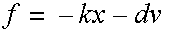
where k is the spring constant and d is the damping. The larger the damping value, the more the mass is slowed along its path. Too little damping and the mass oscillates around the origin. Intermediate “critical” damping means that the system comes to rest in the shortest time. Too much damping means that the system gradually comes to rest.
Try a damping value of -0.5. The system gradually gains energy going faster and faster. Negative damping corresponds to unstable systems. Such things do occur in real life; for instance, a bridge in certain wind conditions may oscillate until it fails. There is another source of instability which is due to the way we are computing motion. The use of discrete time steps is only an approximation. The smaller the time step the more accurate the solution. The mass overshoots where it should be and experiences a greater restoring force than it should. It then overshoots the other way. Oscillations build up and, for more complex objects, the system shakes itself to pieces. This problem may be overcome in two ways. The first is to decrease the time step: this may be achieved by having many subintervals per frame of animation.
This enhances the accuracy of the animation and is vital for fast moving effects. Unfortunately, the more subintervals used, the more expensive the solution, and this can be prohibitive if large numbers of objects are involved. The instability may be counteracted by increasing the damping in the system. Too much damping will lead to altered behaviour; too little and the system becomes unstable and “blows up.”
Extending to More Dimensions — Animating a Chain
The previous spring example was only in one dimension. Most problems of interest work in two or three dimensions.
A force that varies as a function of the distance between two point masses may be expressed as follows:
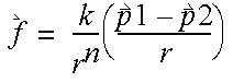
where

and

and

are vectors, and r is the distance between the point masses. n should be set to -1 for a spring, and 2 for gravity.
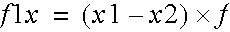
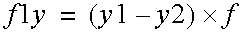
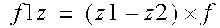
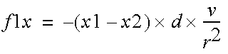
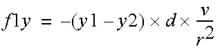
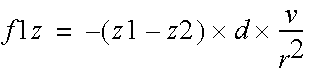
This may be expressed in terms of components as follows:
for points (x1, y1, z1,) and (x2, y2, z2),
The force along x, y, z acting on particle 1 will be:
A damping term should be proportional to relative motion along the line joining the two masses. This may be achieved by computing the dot product of the difference in position with the difference in velocity:

It is possible to have collections of point masses. The position and velocity of each particle is stored in arrays. For each iteration, the cumulative force is computed for each mass pair of interactions.
Cloth or drapery may be simulated using a two dimensional mesh of point masses. These are animated using dynamics and then used to define the control points of a patch. The masses may be considered to be a rectangular mesh in u, v space.
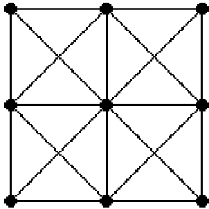
The above illustrates the arrangement of the springs for cloth. Springs run horizontally and vertically to simulate the direct thread properties. Diagonal springs prevent the cloth from shearing.
The constraints holding the top two corners of the cloth move closer together as the animation progresses. Try using larger values of "dbond", the variables which control the shear coefficient. Very large values, such as 1.0 will give a material which behaves more like paper than cloth.
If you intend to render the cloth image, rather than using the wireframe, you should note two things. First, the "divisions" in the patch statement should be increased to three or four. Second, the variable "startframe" should be set to the value of the first frame to be rendered. This is useful if you want to examine just one frame or if you want to restart a render half way through the animation.
Three Dimensional Systems: Jelly and Snakes
Two dimensional sheets are useful for drapery and flags, but often real objects are three dimensional solids. These may be simulated using three dimensional lattices of masses.
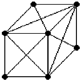
A Cubic Mass - Spring System
A three dimensional lattice will deform when it collides with constraints. It will wobble like a piece of jelly, but it is essentially passive.
A more interesting effect is achievable if the spring tensions are animated with time. This can be used to simulate muscle contractions in biological forms such as worms and snakes. The edge spring lengths are animated sinusoidally to produce sinuous motion in the snake. The directional friction due to the scales is implemented by not permitting the snake to slide backwards. This, and the muscle contractions, cause the snake to slither along. The variable "numxp" controls the number of segments in the snake. A "numxp" of 5 produces a wriggling grub-like motion but is quite fast. A "numxp" of 30 gives a truly convincing snake and takes considerably more time.
As an exercise, try applying a lifting force to one end of the snake and see the resulting movement.


