A detailed comparison of NURBS and Bezier surfaces.
Surface has a common mathematical foundation called b-splines that enable Surface users to generate NURBS geometry (that can imply multi segment geometry) and Bezier geometry (single span geometry).
Mathematically, a single segment NURBS surface is equivalent to a single Bezier surface patch. Mathematically, Bezier surfaces are a subset of NURBS.
Addressing Interior Breaks in Continuity
Using curvature diagnostic functions, users can analyze multi-span degree 3 geometry and detect abrupt changes in G3 curvature.
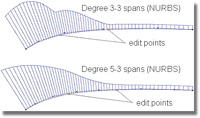
The above image demonstrates the difference in curvature combs when analyzing multi-span degree 3 and degree 5 geometry. The top curve in the above image is a degree 3-3 span curve; notice the abrupt changes in the curvature comb. The lower curve in the above image is a degree 5 curve; the degree 3 curve has been rebuilt to degree 5 without any CV modification. The deviation between the two curves is 0.000 millimeters. The degree 5 curve is just as easy to achieve using Surface.
When to use Bezier Surfaces instead of NURBS Geometry
When using Bezier geometry, each CV has an equal effect on the shape of a curve or surface (curvature comb). When using NURBS geometry, a single CV's influence is limited to a local region of the geometry. This local region is referred to as a span or a segment. In NURBS geometry, these segments are linked together mathematically, but each segment can be modified locally.
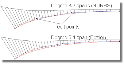
The above image compares Bezier and NURBS geometry. Each curve has seven CVs, offering an equal amount of shape control. The top curve is a NURBS curve while the lower curve is a Bezier curve. Note the highlighted portions of each line; these are the portions of the curve that will be modified when moving the selected CVs. On the NURBS curve, only a portion of the curve is highlighted whereas the entire curve is highlighted on the Bezier curve. This image demonstrates the difference between NURBS and Bezier segmentation.
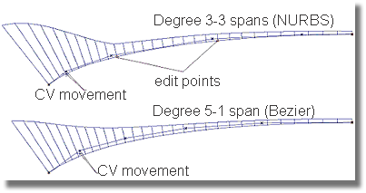
The above image demonstrates the results of a small movement of the CVs selected in the previous image. The CVs on each curve were moved in equal amounts. Notice how the curvature combs have been affected in different manners by the movement of the CVs. While this example suggests that it may be easier to control a curvature comb by using Bezier geometry, Surface users are not necessarily required to use Bezier geometry.
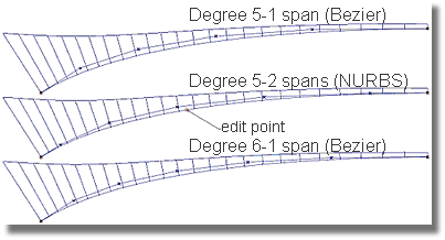
In the above image, Bezier and NURBS geometry are further compared. The three curvature combs in the above image depict a degree 5 curve at the top, a degree 5-2 span curve in the middle, and a degree 6 curve at the bottom. The curves are identical in shape, but vary in complexity. The purpose of the above image is to demonstrate that a NURBS curve can have the same curvature characteristics as a Bezier Curve.
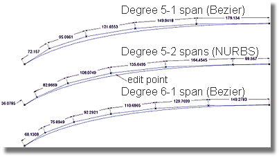
As can be seen in the image above, the difference between the curves depicted in the previous image lies in the spacing of the CVs. As a general rule, Surface users are encouraged to place more CVs where higher areas of curvature are desired. In the example depicted in the image above, the distribution of CVs found in the middle and bottom curves are the result of two different rebuilding methods that were applied to the top curve. When the top curve was originally created, optimal CV distribution was employed, resulting in a gradual decrease in the distances between CVs.
The two rebuilding methods used on the top curve are:
Method 1 (middle curve): rebuild the degree 5 curve to a degree 5-2 span NURBS curve. Note that the spacing of the CVs is no longer decreasing.
Method 2 (bottom curve): rebuild the degree 5 curve to a degree 6 Bezier curve. By increasing the curve's degree, the CV spacing continues to decrease.
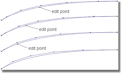
The above image demonstrates the insertion of additional spans into a degree 5 curve. When a user inserts a span in an effort to increase control, it can be difficult to anticipate where the new CVs should be located. This “freehand” type of rebuilding can often lead to CVs being placed too close to one another, or cluttered at, or near, the end of the geometry. This uneven CV distribution may result in rapid curvature changes when the CVs are modified. The addition of CVs is a measure to help gain more control over curves or surfaces, but the uneven distribution of CVs can, as in this example, reduce the amount of control. When using Surface, instead of adding spans, increase the degree of a curve as the modifications will maintain uniform CV distribution.
When to use NURBS Geometry instead of Bezier Geometry
When two surfaces intersect, the resulting curve (intersection line) can be more complicated than either of the two input surfaces. The reason for the increase in complexity is mathematics. In Surface, users set the system tolerances to specify the continuity required along surface boundaries, but to create complex geometric shapes, more control may be required. The shapes produced by Bezier geometry are somewhat limited by the degree value, which in turn, can be limited by the downstream CAD system.
How CAD systems can achieve the required surface boundary tolerances when the degree value can no longer be increased
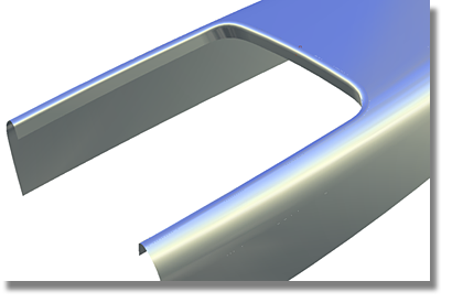
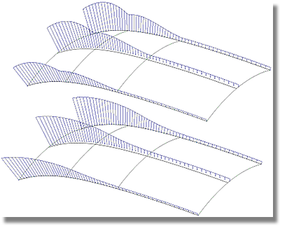
The image above depicts a complex fillet and flange condition where the main slab surfaces are Bezier surfaces. When the small flanges and fillets are constructed, the system requires more complex shapes (more CVs) to maintain the required tolerance.
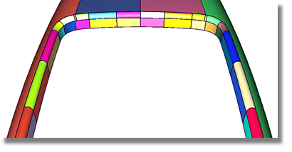
The above image demonstrates how Bezier modeling systems increase the number of CVs while maintaining the tolerance requirements. To approximate complex shapes, additional surfaces are generated. For example, if one degree 5 surface (comprised of 6 CVs) does not meet the edge tolerance, two surfaces are created. The two degree 5 surfaces will have a combined total of 12 CVs along each edge.
Bezier surface (edge)
(Degree + 1) = # of CVs
Downstream CAD users can sometimes specify a degree limit. To achieve a required tolerance, CAD systems can create additional surfaces containing the specified degree, until the edge tolerance conditions are met.
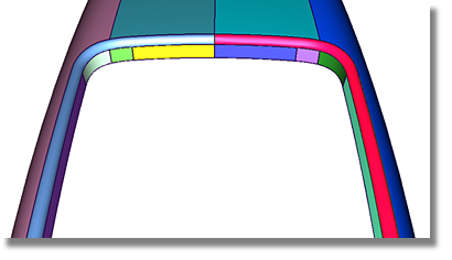
As depicted in the image above, NURBS modeling systems can also solve the tolerance requirements. To create complex shapes, spans are added to each surface until the required tolerances have been meet.
NURBS surface (edge)
(Degree + # of spans) = # of CVs
Using the NURBS method, the degree value remains the same while the number of spans increase. The main benefit of this method is that fewer surfaces are required to define complex shapes.
Choosing the Right Curve for the Job
The popular assumption that degree 5 geometry is superior to other degree geometry is partially true. Degree 5 geometry will not produce internal abrupt G3 changes. But perhaps a better way to look at the advantages of geometic diversity is to consider those shapes other than straight lines and arcs. If users only required parts with straight edges, degree 1 geometry would suffice for all designers. To create more complex shapes, users require higher degrees of geometry, but this does not suggest that all shapes require a degree 5 (or higher) complexity to achieve quality results. There are many techniques that can be employed to create curves in Surface. Two of the main methods are shown in the following images.
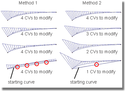
Since the four interior CVs are spaced equally in a straight line at the beginning of the procedure, all four interior CVs must be modified in each step to achieve the final shape.


