X-scans (X-scan lines) are quite different than Y-scans.
Some characteristics of X-scans
Because of the X-scan characteristics, it is possible to model half the model and mirror the other half.
Mirroring saves time, but it can also produce a problem that must be addressed. Running along the Y-plane at the Y0 position, whole surfaces, such as the top surface, are seamless. On the other hand, when employing the “half-side-modeling” method, two surfaces and a connection seam are created. Connection seams lead to modeling problems with curvature combs.
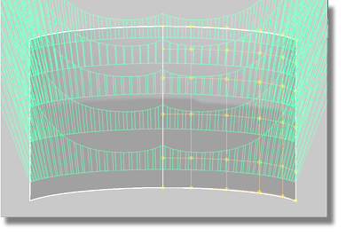
For example, the image below shows a surface that covers the right half of the model. The left half of the model was mirrored from the right half. Note that the curvature combs have a seam crossing the center line. This seam can be modified, but special attention will have to be paid to the manipulation of the surface.
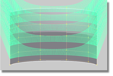
In contrast, the image below shows one surface covering the entire top of the model. The curvature combs crossing the center line are smooth, and as a result, you will never have to check the appearance of the curvature comb crossing the Y0 position.
To avoid the problems created by mirroring, all surfaces that cross the center line should be constructed as one surface.
To fit a curve that crosses the center line
 menu item).
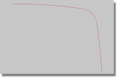
 tool to produce the option
box.
tool in the same manner
as detailed in “Establishing and creating the center line” section.
tool to produce the option
box.
tool in the same manner
as detailed in “Establishing and creating the center line” section.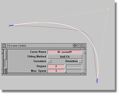
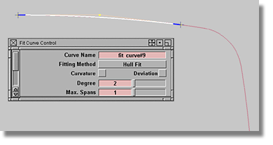
Once you have created the curve and matched it to the scan line, you can use it as a guide.
 .
.
 to produce the Mirror Options box.
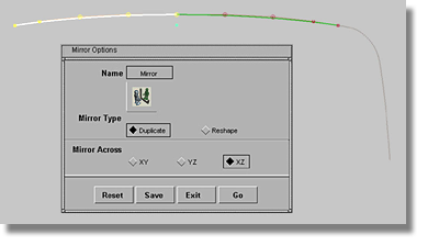
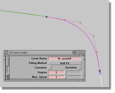
Two points have now been produced, one at either side of the model, each with a corresponding position relative to the center line. The next step in the procedure will be to create the real curve.
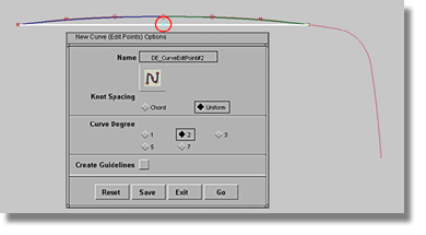
 icon to produce its option box.
| Set this parameter... | To this value |
|---|---|
| Knot spacing | Uniform |
| Curve degree | 2 |
| Create guidelines | off |
.
As you manipulate the CV in the Z-direction, you may notice that you cannot model the shape of the scanned line with just one free CV. Eventually, you will need more CVs, but not before giving some thought to the maximum number of CVs you will require. To tackle this question, always start with the lowest degree (number of CVs) and increase the value in small steps. Employing a lowest-to-highest degree strategy should ensure that you do not overbuild your model.
To increase the number of CVs of a curve
 (Windows) or
  (Mac).
You now have more CVs to help you achieve the shape of the scan line.
With the increase in CVs there is also an increase in the freedom of movement. When moving CVs you should remember to always move corresponding CVs at the same time, otherwise, you will loose the symmetry of the curve.
Going forward with this exercise, you will encounter a problem when trying to change the position of the marked CV in the Y-direction. One solution to this problem is to select the CVs you intend to move on both sides of the center line and then center the pivot point. You will then be free to move the CVs using a non-proportional scale.
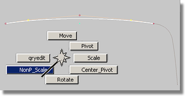
To move CVs using a non-proportional scale
.
You will now be able to fit the curve to the scan line, but don’t consume too much time measuring the deviations between the scan line and the curve. Instead, concentrate on trusting your eyes and developing an understanding of the CVs role.
After completing the top curve, continue creating the missing parts of the X-scan line. Use the same methods you learned when creating the center line (changing the endpoints of the curves, and modifying the blend curve using the manipulator).
Remember to check the
curvature comb of your X-curves by selecting all the curves and
then using the Locators > Curve Curvature  tool.
tool.
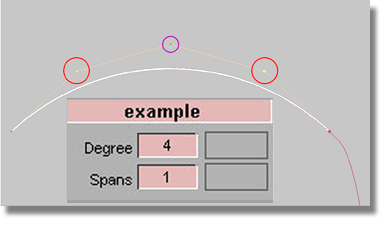
Also, take care when polishing the curvature plot that you limit your movement to the non-proportional scale of the CVs on the top curve. To avoid destroying the symmetry of the curve, you should not use the SLIDE command if the curve runs across the Y0 position.
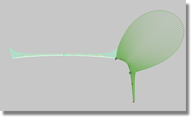
Your efforts should resemble the curve in the image above.
At this point in the tutorial, you should have an empty screen.


